Problem 2.3

Provide two illustrations of how derivatives are applied in real-world scenarios.

One of the most useful application would be license plate Detection
given License plate picture we can perform edge Detection as discussed in previous problem Prewitt-Operator with following steps

transform picture into gray_scale image
calculate convolution
apply filter to detect edges
use threshold to get cleared-view

this is the following result

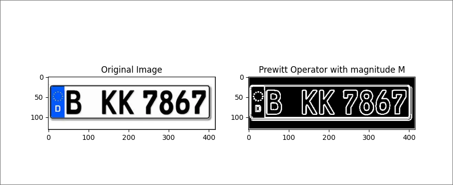
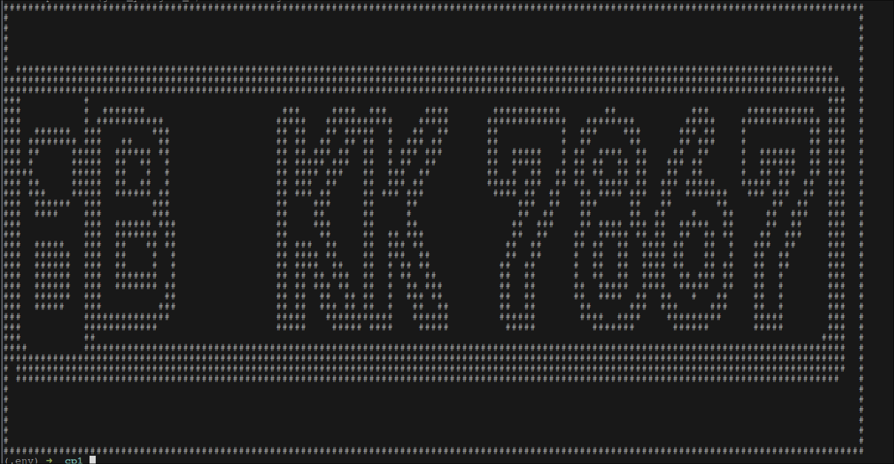
from which we can extract license plate number much easily. simplest solution would be to print some character(i.e #) whenever we encounter
value of 1 (which is the highest value in processed image) in the image matrix.
even with such simple approach we can get pretty good results.

with following implementation

import numpy as np
import skimage.io as io
from skimage.filters import gaussian
import skimage.color as color
import matplotlib
from scipy.signal import convolve

matplotlib.use("TkAgg")

import matplotlib.pyplot as plt


def convert_to_rgb_format(img):
    if img.shape[2] == 4:
        img = color.rgba2rgb(img)
    return img


def convert_to_gray_scale(img):
    return color.rgb2gray(img)


def threshold(g, T):
    h, w = g.shape[:2]
    for j in range(h):
        for i in range(w):
            if g[j, i] >= T:
                g[j, i] = 1
            else:
                g[j, i] = 0
    return g


def extract_characters(image, max_print_size=120):
    m, n = image.shape[:2]

    resolution = min(max_print_size / max(m, n), 1)

    step_size = int(1 / resolution)

    for i in range(0, m, step_size):
        for j in range(0, n, step_size):
            if np.any(image[i : i + step_size, j : j + step_size] == 1):
                print("#", end="")
            else:
                print(" ", end="")
        print()


def prewitt_operator(g):
    h_x = np.array([[1, 0, -1], [1, 0, -1], [1, 0, -1]])
    h_y = np.array([[1, 1, 1], [0, 0, 0], [-1, -1, -1]])

    grad_x = convolve(g, h_x, mode="same")
    grad_y = convolve(g, h_y, mode="same")

    M = np.sqrt(grad_x**2 + grad_y**2)  # NOTE: magnitude M

    A = np.arctan(grad_y / grad_x)  # NOTE: angle A

    return M, A


img = io.imread("./plate.png")

#NOTE: to test gaussing blur
# _img = gaussian(img, sigma=5)

img = convert_to_rgb_format(img)

g = convert_to_gray_scale(img)

M, A = prewitt_operator(g)

M_th = threshold(M, 0.5)

extract_characters(M_th)


plt.figure(figsize=(10, 5))

plt.subplot(1, 2, 1)
plt.imshow(img)
plt.title("Original Image")

plt.subplot(1, 2, 2)
plt.imshow(M_th, cmap="gray")
plt.title("Prewitt Operator with magnitude M")
plt.show()

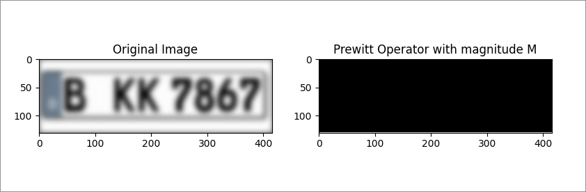
Unsuccessful findings

the drawback of this method is that it is sensitive to image noising. this is the illustration of the same image with Gaussian blurr
with

pics/gaussian.png

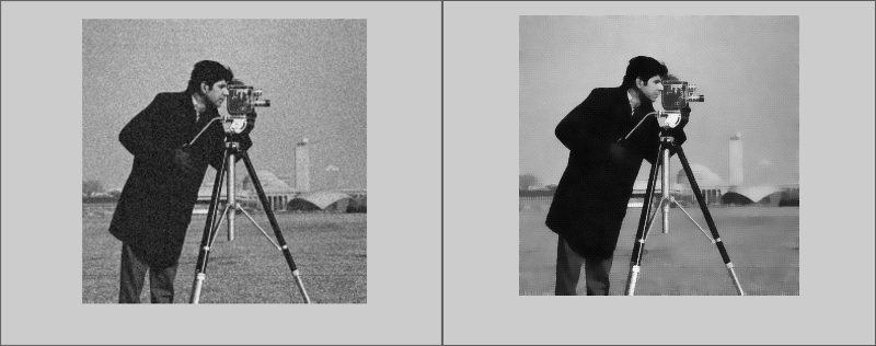
Another application of Derivatives is Image Denoising with Gradient-Descent (GDM)

for typical GDM method would be to minimize some objective function
$𝕞 𝕚 𝕟$ with iteration but in image Denoising instead of minimizing sequence of we look for minimizing sequence of images for functional where V is space of images (space of smooth functions)

We consider functional which are the addition of two terms, . The first term is the fidelity term which forces the final image to be not too far away from the initial image.
The second term is the regularizing term, which performs actually the noise reduction.
A typical choice of the fidelity term is the convex functional

where denotes set of pixels and is the initial image.

For the regularizing term, we start with the simplest choice (also convex)

Then the problem is: find a minimum of solving

to control rate fidelity-regularization.

For using the gradient descent method we need to compute the gradient of . The result is

Then, the gradient descent algorithm gives

this is the illustration of application of GDM on picture.

Problem 2.2 Problem 2.4